
Day 4: Vector Databases - Your AI's Filing Cabinet for a Million Patient Records
RAG for Healthcare | Day 4 of 35 | Free

On Day 3 you learned that embeddings convert text into lists of numbers that represent meaning - and that similar meanings produce similar numbers. Beautiful concept. One problem:
Where do you put a hundred thousand of them? And how do you search through them fast enough for a clinician who needs an answer in seconds, not minutes?
Today you meet FAISS: Facebook AI Similarity Search - the library that powers the retrieval engine behind most production RAG systems. By the end of this article, you will understand how it works, why there are different index types, and which one to choose for your healthcare use case.
The Problem: A Cardiologist With a Needle-in-a-Haystack Question
Your hospital has 100,000 de-identified discharge summaries stored as embeddings - each one a list of 3,072 numbers, exactly as we described on Day 3.
A cardiologist walks up to the system with a complex query:
“68-year-old male with HFrEF, recent ICD implant, presenting with recurrent ICD shocks and hypokalemia.”
Clinical context: let’s unpack every term:
HFrEF (Heart Failure with Reduced Ejection Fraction): The heart muscle is weak and can’t pump forcefully enough. We covered this on Day 3 - ejection fraction below 40% is considered reduced. This patient’s heart is failing.
ICD (Implantable Cardioverter-Defibrillator): A small device surgically placed under the skin, usually below the collarbone, with wires threaded into the heart. It continuously monitors the heart rhythm. If it detects a life-threatening arrhythmia (like ventricular tachycardia or ventricular fibrillation - dangerously fast or chaotic rhythms that can cause sudden death), it delivers an electric shock to reset the heart to normal. Think of it as a tiny, internal emergency defibrillator that’s always on watch.
Recurrent ICD shocks: The device keeps firing - delivering painful electric jolts to the patient’s chest. This means the patient’s heart keeps going into dangerous rhythms, over and over. This is a medical emergency. It’s terrifying for the patient and indicates a serious underlying problem that needs urgent treatment.
Hypokalemia: Low potassium in the blood (normal is 3.5–5.0 mEq/L). This is critically important here because potassium directly controls the electrical stability of heart cells. When potassium drops too low, the heart becomes electrically unstable - which triggers exactly the kind of dangerous arrhythmias the ICD is shocking. So in this case, the hypokalemia is likely causing the recurrent shocks. Fix the potassium, and you may stop the arrhythmia storm.
The clinical picture: This is a very sick patient with a weak heart, whose ICD keeps shocking him because his low potassium is making his heart electrically unstable. The cardiologist needs to find similar cases - fast - to see what worked.
The system needs to search all 100,000 embeddings and return the 5 most semantically similar discharge summaries. And it needs to do this in under 50 milliseconds - because clinical decisions don’t wait.
This is what FAISS does.
What Is FAISS?
FAISS stands for Facebook AI Similarity Search. It’s an open-source library developed by Meta AI Research that does one thing extraordinarily well: finds the most similar vectors in a large collection, fast.
You give FAISS a collection of vectors (your document embeddings) and a query vector (your question’s embedding). FAISS returns the vectors closest to your query - the nearest neighbors.
The analogy: Think of a massive hospital medical records room with 100,000 patient charts. You walk in and say, “Find me charts most similar to this patient.” A human librarian would take days. FAISS is like having a librarian with a photographic memory and a perfectly organized filing system who can scan all 100,000 charts and hand you the 5 best matches in the time it takes to blink.
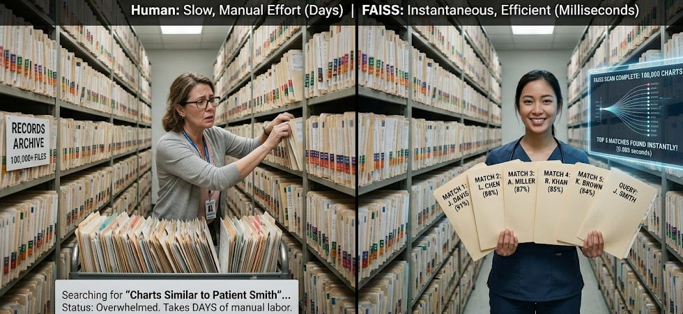
But here’s the key insight: how you organize the filing system determines how fast the search is. And that’s where FAISS index types come in.
The Three Filing Systems: Flat, IVF, and HNSW
FAISS offers several index types. Each one is a different strategy for organizing your vectors so they can be searched efficiently. Think of them as three different ways to organize that medical records room
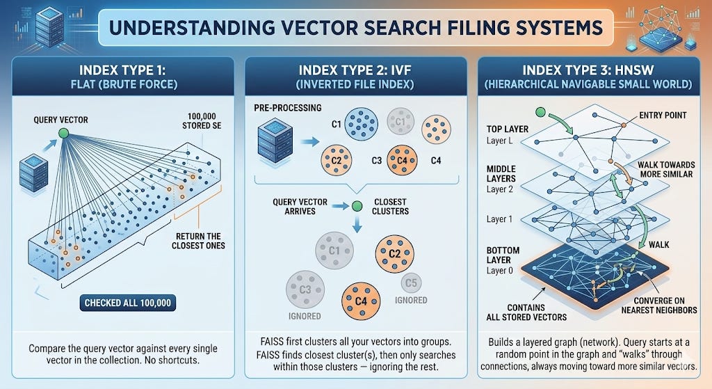
Index Type 1: Flat (Brute Force)
How it works: Compare the query vector against every single vector in the collection. No shortcuts. Check all 100,000. Return the closest ones.
The analogy: You walk into the records room and literally open every single one of the 100,000 folders, compare each one to your query, and rank them all. You will find the best matches - guaranteed - but it takes a while.
Strengths:
Perfect accuracy. Because you check everything, you’re guaranteed to find the true nearest neighbors. No approximation.
Simple. Nothing to configure. No tuning parameters.
Weaknesses:
Slow at scale. Checking every vector is fine for 1,000 documents. For 100,000, it’s getting slow. For 10 million, it’s impractical.
When to use it in healthcare:
Prototyping and development (your first RAG system: which you’ll build on Day 7)
Small document collections (under ~50,000 vectors)
When accuracy is absolutely critical and speed is secondary: like a research study where you need guaranteed best matches
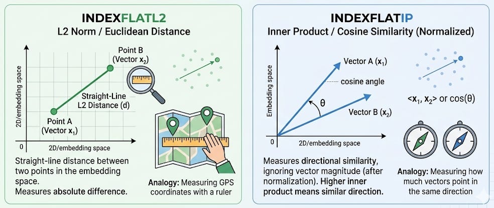
The technical detail: FAISS calls this IndexFlatL2 (using L2/Euclidean distance) or IndexFlatIP (using inner product, which relates to cosine similarity). The “L2” stands for L2 norm: the straight-line distance between two points in the embedding space. Think of it like measuring the distance between two GPS coordinates with a ruler on a map.
Index Type 2: IVF (Inverted File Index)
How it works: Before searching, FAISS first clusters all your vectors into groups of similar vectors. When a query comes in, FAISS first figures out which cluster(s) the query is closest to, and then only searches within those clusters - ignoring the rest.
The analogy: Instead of one giant records room, you’ve reorganized it into departments: a cardiology wing, a neurology wing, a pulmonology wing, and so on. When a query about heart failure comes in, you walk straight to the cardiology wing and only search those charts. You skip neurology, pulmonology, and everything else. You search maybe 5,000 charts instead of 100,000.
Clinical context for why this matters: In a hospital, clinical cases naturally cluster. Heart failure patients have discharge summaries that are semantically similar to each other. Sepsis patients cluster together. Stroke patients cluster together. IVF exploits this natural clustering to dramatically speed up search.
Strengths:
Much faster. Typically 10–20x faster than Flat at scale, because you’re only searching a fraction of the data.
Configurable trade-off. You control how many clusters to search (
nprobe). Search more clusters = more accurate but slower. Search fewer = faster but might miss a relevant document in a neighboring cluster.
Weaknesses:
Approximate. Because you skip some clusters, you might miss a relevant document that happened to be placed in a cluster you didn’t search. In practice, searching 5–10% of clusters typically recovers 95%+ of the true nearest neighbors.
Requires training. You need to build the clusters before you can search, which takes a one-time upfront computation.
When to use it in healthcare:
Medium to large document collections (50,000 to several million)
Clinical search where near-perfect accuracy with 10x speed improvement is a good trade-off
Most production healthcare RAG systems
The technical detail: FAISS calls this IndexIVFFlat. The “inverted file” name comes from information retrieval - it’s an index that maps from cluster centroids back to the documents in each cluster, similar to how a book index maps from a topic back to page numbers.
Index Type 3: HNSW (Hierarchical Navigable Small World)
How it works: FAISS builds a graph - a network where each vector is connected to its nearby neighbors. When a query comes in, the search starts at a random point in the graph and “walks” through the connections, always moving toward more similar vectors, until it converges on the nearest neighbors.
The analogy: Imagine you’re in a new hospital and you need to find the cardiology department. You don’t have a map. But you can ask anyone for directions. You ask the receptionist (random starting point) - she says “go to the third floor.” On the third floor, you ask a nurse - she says “turn left, it’s near the echo lab.” At the echo lab, someone says “next door.” Each step gets you closer. You find it quickly, not by searching the whole building, but by following increasingly specific directions through a network of people.
That’s HNSW. Each “person” is a vector, each “direction” is a graph edge connecting similar vectors, and the “asking” is computing similarity between the query and each connected neighbor.
Why “Hierarchical”? The graph has multiple layers - like having guides on every floor of the hospital. The top layer has few nodes and makes big jumps (like “go to the third floor”). Lower layers have more nodes and make fine-grained jumps (like “two doors down on the left”). This hierarchy lets the search start with coarse navigation and progressively zoom in.
Strengths:
Extremely fast. Often the fastest option for real-time search.
No separate training step. Vectors are added to the graph incrementally.
Great recall. Typically finds 95–99% of true nearest neighbors.
Weaknesses:
Uses more memory. The graph connections require additional storage - roughly 2–4x more memory than a Flat index for the same data.
Complex to tune. Parameters like
M(connections per node) andefConstruction(build quality) affect both speed and accuracy.
When to use it in healthcare:
Real-time clinical search applications where speed is critical
Large-scale systems (millions of documents)
When you can afford the extra memory
The technical detail: FAISS calls this IndexHNSWFlat. The “Small World” part of the name comes from network science - the idea that in well-connected networks, any two nodes can be reached in a small number of steps (like the “six degrees of separation” concept).
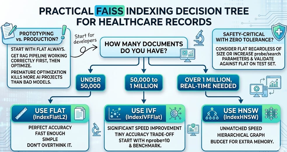
How to Choose: The Decision Framework
Here’s the practical decision tree for healthcare:
The Complete Flow: From Clinical Document to Search Result
Let’s trace the entire journey from a clinical document to a search result, connecting Day 3 and Day 4:
Ingestion (done once):
Take a discharge summary: “68-year-old male admitted for recurrent ICD shocks in the setting of hypokalemia. History of ischemic cardiomyopathy with LVEF 20%. Potassium was repleted to 4.2 mEq/L, amiodarone was initiated, and ICD interrogation confirmed appropriate shocks for ventricular tachycardia…”
Convert it to an embedding: a list of 3,072 numbers representing its meaning (Day 3).
Add that embedding to the FAISS index, along with metadata (the document ID, patient ID, date, etc.) so you can retrieve the original text later.
Repeat for all 100,000 discharge summaries.
Clinical context on the ingestion example: Ischemic cardiomyopathy means the heart muscle is damaged from blocked coronary arteries (past heart attacks). LVEF 20% is severely reduced - the heart is very weak. “Potassium was repleted” means they gave the patient potassium supplements to bring the level back to normal. Amiodarone is a powerful antiarrhythmic drug (we met it on Day 1) used here to suppress the dangerous rhythms. “ICD interrogation” means a technician wirelessly downloaded the device’s stored data to review what rhythms triggered the shocks. “Appropriate shocks” means the ICD correctly identified a life-threatening rhythm - it did its job.
Search (done every query):
The cardiologist types a query.
Convert the query to an embedding using the same model.
FAISS searches the index and returns the 5 nearest neighbors - the 5 discharge summaries whose embeddings are closest to the query’s embedding.
Those 5 documents get passed to the generator (the LLM), which synthesizes an answer grounded in real clinical evidence.
That’s it. That’s the retrieval pipeline from Day 1, now fully demystified.
FAISS vs. Other Vector Databases
FAISS is a library, not a database server. This is an important distinction. It runs in your Python process, stores indexes in local files, and has no built-in networking, authentication, or multi-user access.
For production healthcare systems, you may eventually want a managed vector database that adds those features. The major options in 2026:
FAISS (library): Free, fast, runs locally. Perfect for prototyping and single-user applications. What we’ll use throughout this series.
Pinecone (managed service): Hosted, scalable, easy to use. Vectors leave your infrastructure - important to consider for PHI.
Weaviate (open-source or managed): Supports hybrid search (keyword + semantic). Can be self-hosted for HIPAA compliance.
Qdrant (open-source or managed): Strong filtering capabilities. Can be self-hosted.
ChromaDB (open-source): Lightweight, developer-friendly. Good for prototyping.
pgvector (PostgreSQL extension): If you’re already using PostgreSQL, this adds vector search without a new tool.
For this series, we use FAISS. It’s the right choice for learning because there’s no infrastructure to set up, no accounts to create, and no cost. Everything runs in your Google Colab notebook. When you’re ready to scale to production, the concepts transfer directly - the embeddings are the same, the search is the same, only the storage layer changes.
What Vector Databases Do NOT Do
Staying consistent with our intellectual honesty:
They don’t understand your query. The vector database is pure math - it computes distances between vectors. It doesn’t “know” that hypokalemia causes arrhythmias or that ICD shocks indicate electrical instability. All of that understanding lives in the embeddings (created by the embedding model) and the generator (the LLM). FAISS is just the filing cabinet.
They don’t filter by metadata natively (in basic FAISS). If you want “find similar cases, but only from patients over 65” or “only from the last 2 years,” basic FAISS can’t do that. You need to either pre-filter your data before searching or use a vector database with built-in metadata filtering (we’ll cover this on Day 19).
They don’t guarantee clinical relevance. The 5 most mathematically similar embeddings may not be the 5 most clinically useful documents. A discharge summary about a patient with recurrent ICD shocks from lead fracture (a mechanical problem with the device wire) is semantically similar to our query but clinically a very different situation than shocks from hypokalemia. This is why reranking (Day 13) and metadata filtering (Day 19) exist.
Your Takeaway for Today
A vector database stores embeddings and finds the most similar ones to a query - fast. FAISS is the most widely used library for this. Choose Flat for small datasets and prototyping, IVF for medium/large, and HNSW for real-time search at massive scale.
The retriever from Day 1 is no longer a mystery. You now know what goes into it (embeddings, Day 3), where they’re stored (vector database, today), and how the search works (nearest neighbor search over vectors). The next question is: how do you prepare your clinical documents so the embeddings are actually good?
Coming Tomorrow: Day 5
Chunking - How You Split Clinical Documents Changes Everything
You can’t embed a 30-page discharge summary as a single vector - too much meaning crammed into one point, and the important details get diluted. Tomorrow you’ll learn how to split medical records into chunks that preserve clinical meaning, and why the wrong chunking strategy can make your RAG system useless even with perfect embeddings and a perfect index.
→ Subscribe to RAG for Healthcare so you don’t miss Day 5.
Teodora Szasz, PhD - Senior Clinical Data Scientist | FDA 510(k) AI | Co-author, EchoJEPA