

Watch the video above.
Below: the full story of a design choice that changed our AI model’s performance by 26.7% - and what it teaches about building AI that actually works in the real world.
Last episode I explained self-supervised learning - hide part of the data, predict what’s missing, learn from the process. Simple, elegant, powerful.
But I left you with a teaser: WHAT you predict matters as much as the prediction itself.
This episode is the payoff. And it’s personal - this is the single design decision we are most proud of in building EchoJEPA.
Two art students and a photograph
Let me start with an analogy.
Imagine two art students. You show both of them a photograph with a section cut out, and you ask them to fill in the missing area.
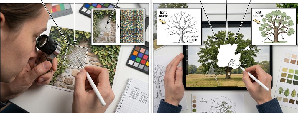
Student A is meticulous. They study the surrounding pixels, the exact color values, the grain of the paper, every tiny imperfection - and try to reproduce the missing region as a pixel-perfect copy. If there’s a smudge on the lens, they reproduce the smudge. If there’s film grain, they reproduce the grain.
Student B takes a different approach. They look at the scene and think: “OK, there’s a tree here, the light source is to the left, the leaves are this shade of green, there’s a shadow at this angle.” Then they fill in the missing region based on their understanding of what’s IN the image - the objects, the structure, the relationships.
Student A works in pixel space - predicting the literal surface values. Student B works in latent space - predicting the meaning behind the surface.
For a clean, high-quality photograph, both students do well. The difference is barely noticeable.
But now give them a noisy image. And watch what happens.
The noise problem in ultrasound
Echocardiography (heart ultrasound) is not like a photograph. Every ultrasound image contains speckle noise: a shimmering, grainy texture that’s fundamental to how ultrasound physics works. Sound waves bounce off tissue, interfere with each other, and create patterns that look random.
 - Dysautonomia-MVP Center - Paula ...")
And crucially: speckle IS random. It’s different in every single frame, even when the heart underneath is in the exact same position doing the exact same thing. Frame 1 and frame 2 might show the same ventricle, but the speckle pattern is completely different.
This creates a problem for Student A - the pixel predictor.
When you ask a model to predict the exact pixel values of a masked region in an ultrasound image, the model MUST reproduce the speckle noise. It’s part of the pixels. The model can’t distinguish “these pixels represent the heart wall” from “these pixels represent random speckle.” It’s all just numbers.
So the model dedicates significant capacity - significant learning - to modeling the patterns in randomness. It tries to learn the structure of noise.
It’s like asking someone to memorize TV static. There’s nothing to memorize. But the model will try.
The result: a model that’s mediocre at understanding hearts because it spent too much of its learning budget on understanding noise.
Student B: predict in latent space
Our solution was to become Student B. Don’t predict pixels. Predict in latent space: compressed, meaningful representations that capture what’s in the image rather than what the image literally looks like.
This is the JEPA approach: Joint-Embedding Predictive Architecture.
Here’s how it works mechanically. We have two encoders:
The main encoder: this is the model we’re training. It processes the visible (unmasked) parts of the video and tries to predict representations of the masked parts.
The target encoder: this processes the full video (including the masked parts) and produces the “correct answer” the main encoder is trying to match.
The target encoder is an EMA (Exponential Moving Average) of the main encoder. Instead of being trained directly, it’s updated as a running average of the main encoder’s weights over thousands of training steps.
This detail sounds minor. It’s the whole game.
Why averaging kills noise and preserves signal
Here’s the key insight: and once you see it, you can’t unsee it.
Speckle noise is random. In frame 1, a particular pixel might be bright due to noise. In frame 2, that same pixel might be dark. In frame 3, medium. Over thousands of frames, the noise at any given location varies randomly around some average value.
When the EMA target encoder averages over thousands of training steps, each step processing different frames with different noise patterns, the random variations cancel out. Noise that’s different every time averages toward zero.
But the heart is consistent. The left ventricle wall is in the same place, frame after frame. It contracts and relaxes in the same pattern. The valve opens and closes at the same position. Consistent structure, repeated across every frame, accumulates through averaging. It gets reinforced.
The EMA target encoder produces representations where the noise has been naturally smoothed away and the anatomy has been naturally amplified. Clean, stable descriptions of cardiac structure - for free, through the mathematics of averaging.
When we train the main encoder to predict these clean targets from noisy inputs, it learns: “ignore the noise, find the structure.” It learns to extract meaning from messy data. It learns hearts.
The evidence
Theory is nice. Numbers are better.
Accuracy: On estimating left ventricular ejection fraction (the single most important measurement in clinical cardiology) our JEPA approach outperformed the Masked Autoencoder (pixel prediction) baseline by 26.7%. Not a marginal improvement. A generational leap.
Robustness: We deliberately degraded image quality to simulate real-world conditions - poor acoustic windows, probe movement, patient habitus issues. Our model showed 2.3% performance degradation. The best pixel-level baseline showed 16.8%. Our approach was 86% less sensitive to image quality.
Transfer: Trained entirely on adult echocardiography. Tested on pediatric hearts (different size, different proportions, faster heart rates). Zero additional training. Mean absolute error: 4.32 (ours) versus 5.10 (baseline). The foundation transferred to a population it had never seen.
Attention visualization: When we mapped where the model focuses its attention, it consistently localized on cardiac structures - chambers, valves, walls - not image artifacts or noise. The model learned anatomy. Evidence that it learned the right thing.
The broader principle
This extends far beyond heart ultrasound. Any time your data has noise, irrelevant variation, or messy real-world conditions (which is almost all real-world data) the choice of what you predict matters enormously.
Manufacturing images have lighting variation. Satellite images have atmospheric distortion. Audio recordings have background noise. Medical images have scanner-specific artifacts.
In every case, predicting raw pixel values forces the model to model the mess. Predicting in a cleaned-up latent space focuses the model on what matters.
It’s a design philosophy: don’t ask the model to learn everything. Ask it to learn what’s important.
The one thing to remember
The space you predict in determines what the model learns.
Predict pixels and you learn the surface - including all the noise, artifacts, and irrelevant variation. Predict meaning and you learn the structure - the anatomy, the patterns, the relationships that actually matter.
Sometimes the most important decision in building an AI system isn’t the architecture, the dataset, or the compute budget. It’s what you ask the model to do.
Next up: We keep saying “words go in” and “patches go in.” But HOW does data actually enter a Transformer? What IS a token? The answer is simpler than you think - and it explains some weird things about AI you have probably noticed.
I’m Teodora - AI/ML scientist and co-author on EchoJEPA. This design decision - latent prediction over pixel prediction - is the one I’m most proud of. Subscribe to Standout Systems for more.


