
The One Algorithm That Powers All of AI (And It's Embarrassingly Simple)
Gradient Descent: The 200-year-old math trick that taught machines to see, speak, and think — explained so you'll never forget it.

Every AI breakthrough you’ve heard of — ChatGPT, DALL-E, AlphaFold, Tesla Autopilot — runs on the same algorithm.
Not transformers. Not attention. Not neural networks.
Gradient descent.
It’s the engine beneath everything. And it’s so simple, a 19th-century mathematician figured it out with pen and paper.
Yet when I ask ML candidates “How does a neural network actually learn?”, most fumble.
Today, I’m going to make that impossible for you.
The Blindfolded Mountain Climber
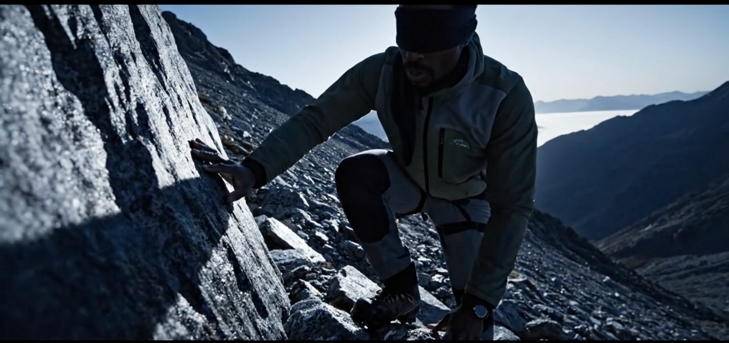
Imagine you’re blindfolded on a mountain. Your goal: reach the lowest valley.
You can’t see anything. But you can feel the ground beneath your feet.
What do you do?
You feel which direction slopes downward, and you take a step that way.
Then you feel again. Step again. Repeat until the ground is flat in every direction — you’ve found the valley.
That’s gradient descent. That’s how every neural network learns.
The “mountain” is the error landscape. The “valley” is where errors are minimized. And “feeling the slope” is computing the gradient.
That’s it. That’s the entire algorithm that powers modern AI.
The Math (Don’t Skip This — It’s Easier Than You Think)
Here’s gradient descent in one equation:
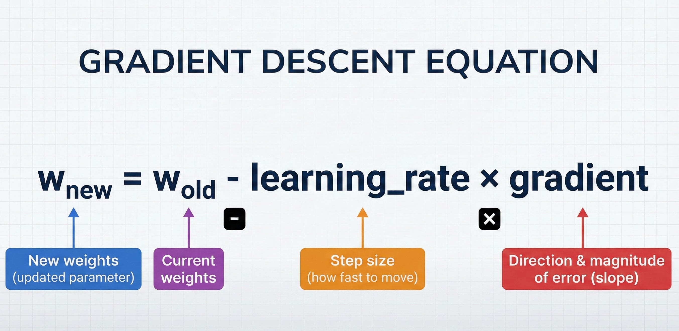
Let me decode this:
w = the model’s weights (what the network is learning) gradient = which direction increases error the most learning_rate = how big a step to take minus sign = go in the opposite direction (downhill, not uphill)
That’s the entire algorithm. Update weights by moving opposite to the gradient.
In code:
python
for epoch in range(num_epochs):
    predictions = model(X)
    loss = compute_loss(predictions, y)
    gradient = compute_gradient(loss, weights)
    weights = weights - learning_rate * gradient
Four lines. This is how ChatGPT learned to write poetry. How Tesla learned to see stop signs. How AlphaFold learned to predict protein structures.
Why Does This Work? (The Intuition)
The gradient tells you: “If I increase this weight slightly, how much does my error increase?”
If the gradient is positive → increasing the weight increases error → so decrease the weight If the gradient is negative → increasing the weight decreases error → so increase the weight
You’re always moving toward lower error. Always rolling downhill.
Do this millions of times across millions of weights, and you get a model that works.
The Three Flavors of Gradient Descent
1. Batch Gradient Descent (The Purist)
Compute the gradient using all training data, then update once.
python
gradient = compute_gradient(ALL_data)
weights = weights - learning_rate * gradientPros: Stable, guaranteed to converge (for convex problems) Cons: Impossibly slow for large datasets. Computing the gradient over millions of examples takes forever.
When to use: Small datasets, when you need precision
2. Stochastic Gradient Descent / SGD (The Speedster)
Compute the gradient using one random training example, then update.
python
for sample in training_data:
    gradient = compute_gradient(sample)  # Just ONE example
weights = weights - learning_rate * gradientPros: Fast updates, can escape local minima due to noise Cons: Noisy, updates jump around a lot
When to use: When you need speed and can tolerate noise
3. Mini-Batch Gradient Descent (The Sweet Spot)
Compute the gradient using a small batch of examples (e.g., 32, 64, 128).
python
for batch in create_batches(training_data, batch_size=64):
    gradient = compute_gradient(batch)  # 64 examples
weights = weights - learning_rate * gradientPros: Best of both worlds — stable enough, fast enough Cons: Batch size is another hyperparameter to tune
When to use: Almost always. This is the default in deep learning.
Interview Gold: “In practice, I’d use mini-batch gradient descent with a batch size of 32-128. It’s more stable than pure SGD but scalable unlike batch gradient descent. Most modern frameworks like PyTorch default to this.”
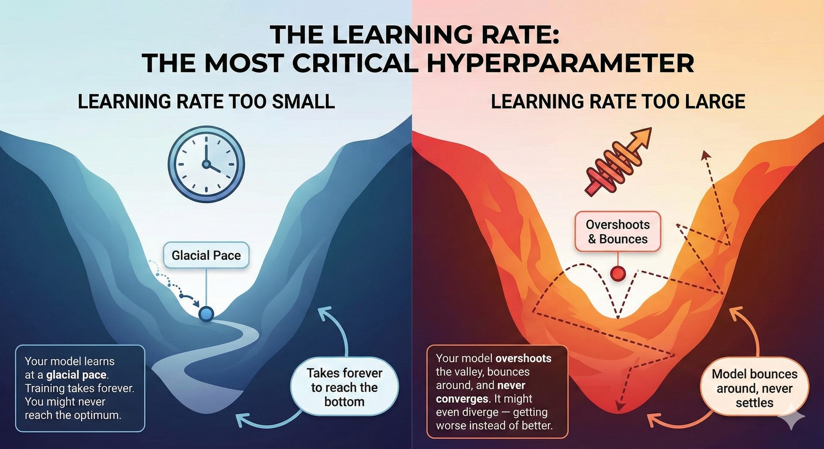
The Learning Rate: The Most Important Hyperparameter You’ll Ever Tune
The learning rate is the single most important hyperparameter in deep learning.
Too small: Your model learns at a glacial pace. Training takes forever. You might never reach the optimum.
Too large: Your model overshoots the valley, bounces around, and never converges. It might even diverge — getting worse instead of better.
The Sweet Spot:
Start with 0.001 or 0.01 (common defaults)
If loss isn’t decreasing, try larger
If loss is jumping around wildly, try smaller
Use learning rate schedulers to decrease over time
Interview Gold: “I’d start with a learning rate of 1e-3, monitor the training loss, and use a scheduler like ReduceLROnPlateau to decrease the learning rate when progress stalls.”
Backpropagation: How the Gradient Actually Gets Computed
Here’s where most explanations lose people. But it’s actually beautiful.
Neural networks are compositions of functions:
Input → Layer 1 → Layer 2 → Layer 3 → Output
         ↑          ↑          ↑
        f₁(x)      f₂(x)      f₃(x)
The output is: y = f₃(f₂(f₁(x)))
To compute how the error changes with respect to each weight, we use the chain rule from calculus:
∂Error     ∂Error    ∂f₃     ∂f₂    ∂f₁
------- = -------- × ---- × ---- × ----
∂w₁       ∂output    ∂f₂     ∂f₁    ∂w₁
This is backpropagation: starting from the error at the output, we propagate the gradient backward through each layer using the chain rule.
Why “back”? Because we start at the end (the error) and work backward to each weight.
Input → Layer 1 → Layer 2 → Layer 3 → Output → Error
                                          ↓
        ←←←←←← Gradients flow backward ←←←←←←
Interview Gold: “Backpropagation is just the chain rule applied systematically. We compute the error at the output, then propagate gradients backward layer by layer. The computational cost is roughly 2-5x the forward pass — this is the Baur-Strassen theorem.”
The 5 Reasons Gradient Descent Can Fail (And How to Fix Them)
1. Stuck in Local Minima
Problem: The algorithm finds a valley, but it’s not the deepest valley.
Solution:
Use momentum (keeps moving even when gradient is small)
Try different random initializations
Use SGD noise to escape shallow minima
2. Vanishing Gradients
Problem: In deep networks, gradients get multiplied many times and shrink to nearly zero. Early layers stop learning.
Solution:
Use ReLU activation (doesn’t squish gradients like sigmoid)
Use batch normalization
Use residual connections (ResNets)
3. Exploding Gradients
Problem: Gradients get multiplied and grow to infinity. Weights become NaN.
Solution:
Gradient clipping (cap the maximum gradient value)
Proper weight initialization (Xavier, He)
Batch normalization
4. Saddle Points
Problem: Points where the gradient is zero but it’s not a minimum — you’re at a plateau.
Solution:
Momentum-based optimizers (Adam, RMSprop)
Add noise via SGD
Larger batch sizes can help
5. Wrong Learning Rate
Problem: Too big = divergence, too small = no progress.
Solution:
Learning rate warmup (start small, increase)
Learning rate scheduling (decay over time)
Adaptive optimizers like Adam
Modern Optimizers: Adam and Friends
Pure gradient descent is rarely used today. Instead, we use adaptive optimizers that automatically adjust the learning rate:
Adam (Adaptive Moment Estimation)
Adam combines two ideas:
Momentum: Keep moving in the same direction (like a ball rolling downhill)
Adaptive learning rates: Different learning rates for different weights
python
optimizer = torch.optim.Adam(model.parameters(), lr=0.001)When to use: Default choice for most deep learning tasks.
SGD with Momentum
python
optimizer = torch.optim.SGD(model.parameters(), lr=0.01, momentum=0.9)When to use: Often works better than Adam for image classification (CNNs). Requires more tuning but can find better solutions.
Interview Gold: “I’d start with Adam for its robustness, but for computer vision tasks, I’d also try SGD with momentum since it often generalizes better. Adam converges faster, but SGD sometimes finds flatter minima that generalize better.”
The Interview Framework
When asked “Explain how neural networks learn” or “Walk me through gradient descent”:
Step 1: The intuition “Neural networks learn by iteratively adjusting weights to minimize error. Gradient descent is the optimization algorithm that does this — it computes which direction to adjust each weight and takes a step in that direction.”
Step 2: The algorithm “We compute the gradient of the loss with respect to each weight using backpropagation — which is just the chain rule. Then we update: new_weight = old_weight - learning_rate × gradient.”
Step 3: The variants “In practice, we use mini-batch gradient descent — computing gradients over small batches of 32-128 examples. This balances stability and speed.”
Step 4: The challenges “Key challenges include choosing the right learning rate, avoiding local minima, and handling vanishing/exploding gradients. Modern solutions include adaptive optimizers like Adam and architectural innovations like residual connections.”
Step 5: The practical choice “For most tasks, I’d start with Adam optimizer, learning rate 1e-3, and batch size 32-64, then tune based on validation performance.”
The Code You Should Know Cold
python
import torch
import torch.nn as nn

# Define model
model = nn.Sequential(
    nn.Linear(784, 128),
    nn.ReLU(),
    nn.Linear(128, 10)
)

# Define optimizer
optimizer = torch.optim.Adam(model.parameters(), lr=0.001)

# Training loop
for epoch in range(num_epochs):
    for batch_X, batch_y in dataloader:

        # Forward pass
        predictions = model(batch_X)
        loss = nn.CrossEntropyLoss()(predictions, batch_y)

        # Backward pass (compute gradients via backprop)
        optimizer.zero_grad()  # Clear old gradients
        loss.backward()        # Compute new gradients

        # Update weights (gradient descent step)
        optimizer.step()
This is the skeleton of every deep learning training loop. Memorize it.
Your Action Items
This week: Implement linear regression with gradient descent from scratch (no frameworks). Feel the algorithm in your bones.
Experiment: Train the same model with learning rates of 0.1, 0.01, 0.001, 0.0001. Watch how training curves change.
Visualize: Plot a 2D loss surface and watch gradient descent navigate it. You’ll never forget how it works.
Interview prep: When they ask “How does a neural network learn?”, your answer should flow: intuition → algorithm → variants → challenges → practical choices.
The Bottom Line
Every AI model you’ve ever used learned through gradient descent.
It’s not glamorous. It’s not complex. It’s a blindfolded climber feeling their way downhill, one step at a time.
But executed billions of times across billions of parameters, it produces machines that can write, see, reason, and create.
The engineers who truly understand gradient descent don’t just use AI — they build it.
Now you’re one of them.
Found this helpful? Share it with someone learning ML.
Questions? Reply directly — I read every response.
Tomorrow: Transformers Demystified — How ChatGPT actually works, explained without the jargon.
Teodora coaches data scientists and ML engineers to land roles at top tech companies. Learn more at teodora.coach