
Vision Transformers (ViT): How Transformers Conquered Computer Vision (+ Complete Code Provided)
The Revolutionary Architecture That Treats Images Like Language

The Paradigm Shift in Computer Vision
For decades, Convolutional Neural Networks (CNNs) dominated computer vision. AlexNet, VGGNet, ResNet—these architectures defined how machines see. Then, in 2020, a Google Research paper asked a simple question: What if we treated images exactly like text?
The result was the Vision Transformer (ViT), and it changed everything.
ViT demonstrated that the same attention mechanism powering GPT and BERT could achieve state-of-the-art results on image classification—without a single convolution. This wasn’t just an incremental improvement; it was a unification of natural language processing and computer vision under one architectural paradigm.
In this guide, you’ll understand:
Why transformers work for images (the key insight)
The ViT architecture explained step-by-step
Patch embeddings — turning pixels into tokens
Positional encoding for 2D images
How ViT compares to CNNs (and when to use each)
The ViT family — DeiT, Swin, BEiT and beyond
Let’s see how transformers learned to see.
Part 1: The Key Insight — Images as Sequences
The Problem with Processing Images
An image is fundamentally different from text:
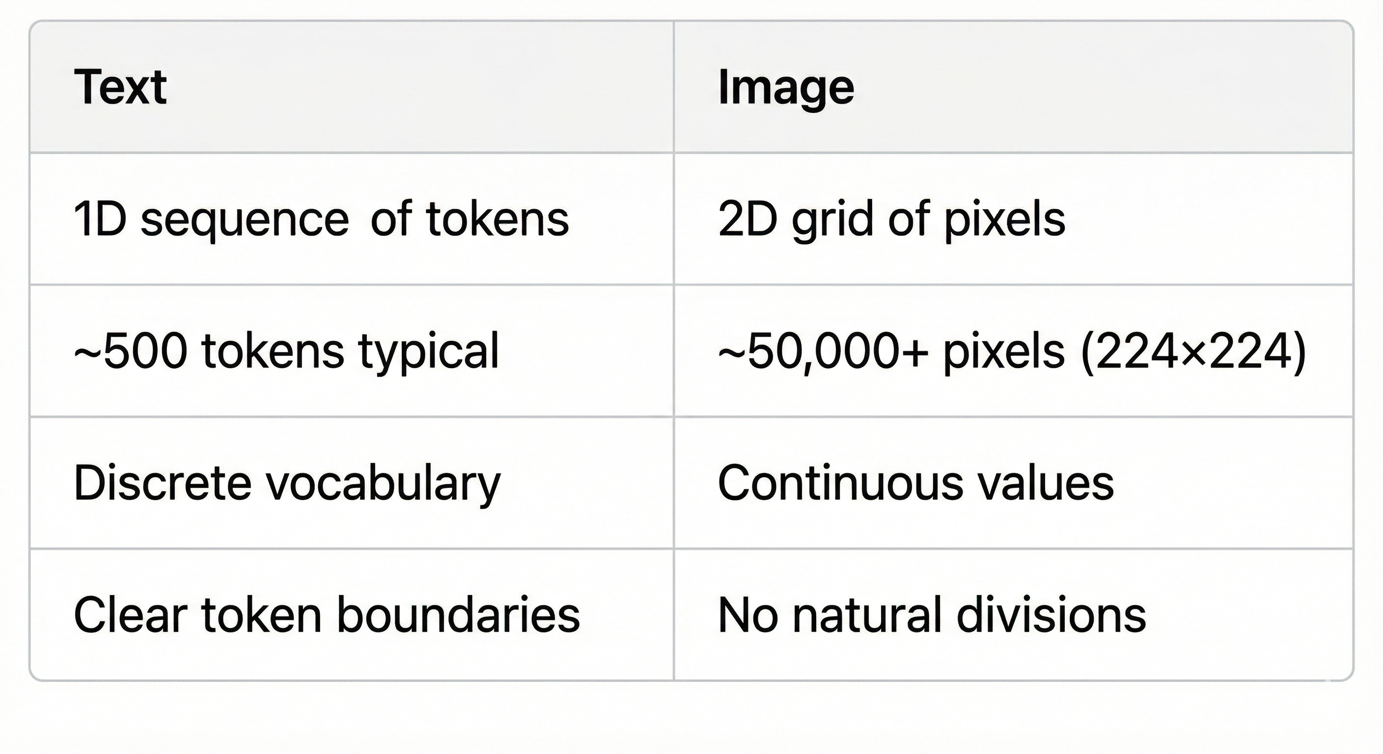
Processing every pixel with attention would be computationally impossible. For a 224×224 image, that’s 50,176 pixels. Self-attention has O(n²) complexity, meaning we’d need to compute over 2.5 billion attention weights per layer.
The Solution: Patch-Based Tokenization
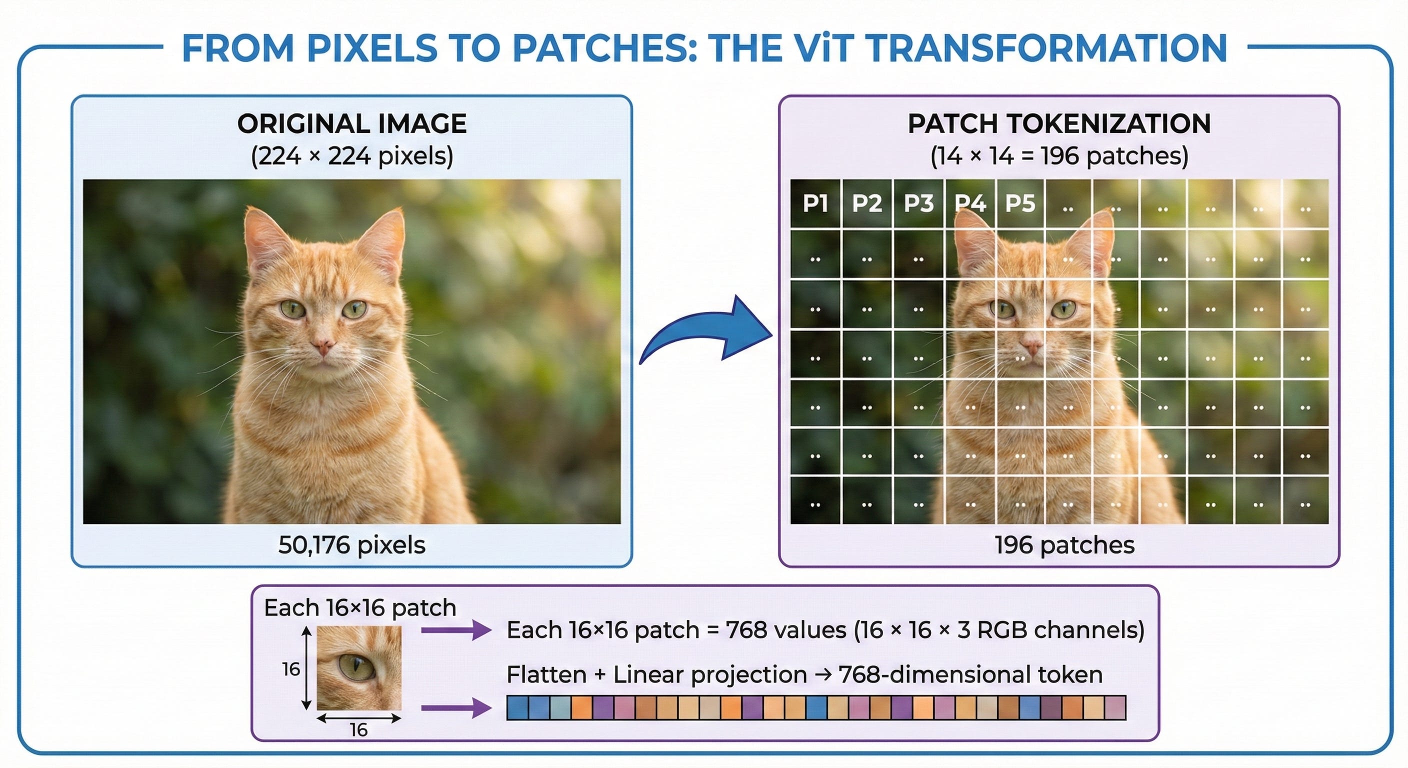
The ViT team’s insight was elegant: don’t process pixels—process patches.
Instead of treating each pixel as a token, divide the image into fixed-size patches (typically 16×16 pixels). A 224×224 image becomes just 196 patches—a manageable sequence length identical to a medium-length text document.
This simple transformation converts computer vision into a sequence modeling problem—exactly what transformers excel at.
Part 2: The ViT Architecture — Step by Step
The Vision Transformer processes images through three distinct stages:
Stage 1: Patch Embedding
The first step converts raw pixels into a sequence of embedded tokens.
Step 1a: Split into Patches
The image is divided into non-overlapping patches of size P×P (typically 16×16):
Input image: H × W × C (e.g., 224 × 224 × 3)
Number of patches: N = (H × W) / P² = (224 × 224) / 256 = 196
Each patch: P × P × C = 16 × 16 × 3 = 768 values
Step 1b: Flatten and Project
Each patch is flattened into a vector and linearly projected to the model dimension D:
Flattened patch: 768 values
After projection: D-dimensional embedding (typically 768)
Projection matrix: Learnable parameters
Step 1c: Add [CLS] Token
A special classification token is prepended to the sequence:
[CLS] token: Learnable D-dimensional vector
Final sequence length: N + 1 = 197 tokens
The [CLS] token aggregates image-level information for classification
Stage 2: Positional Encoding
Unlike CNNs, transformers have no built-in notion of position. Without positional information, the model can’t distinguish between a patch in the top-left corner versus the bottom-right.
